
Anomaly Detection in Time Series using Auto Encoders
In data mining, anomaly detection (also outlier detection) is the identification of items, events or observations which do not conform to an expected pattern or other items in a dataset. Typically the anomalous items will translate to some kind of problem such as bank fraud, a structural defect, medical problems or errors in a text. Anomalies are also referred to as outliers, novelties, noise, deviations and exceptions.
In particular in the context of abuse and network intrusion detection, the interesting objects are often not rare objects, but unexpected bursts in activity. This pattern does not adhere to the common statistical definition of an outlier as a rare object, and many outlier detection methods (in particular unsupervised methods) will fail on such data, unless it has been aggregated appropriately.
Three broad categories of anomaly detection techniques exist:
- Unsupervised anomaly detection techniques detect anomalies in an unlabeled test data set under the assumption that the majority of the instances in the data set are normal by looking for instances that seem to fit least to the remainder of the data set.
- Supervised anomaly detection techniques require a data set that has been labeled as “normal” and “abnormal” and involves training a classifier (the key difference to many other statistical classification problems is the inherent unbalanced nature of outlier detection).
- Semi-supervised anomaly detection techniques construct a model representing normal behavior from a given normal training data set, and then testing the likelihood of a test instance to be generated by the learnt model.
In this article, we will focus on the first category, i.e. unsupervised anomaly detection. The type of algorithm we will use is called auto encoders. Auto encoders provide a very powerful alternative to traditional methods for signal reconstruction and anomaly detection in time series.
Auto Encoders
What is an auto encoder? It is an artificial neural network used for unsupervised learning of efficient codings. Its goal is to induce a representation (encoding) for a set of data by learning an approximation of the identity function of this data \(Id : \mathcal {X} \rightarrow \mathcal {X}\).
Architecturally, the simplest form of an auto-encoder is a feedforward, non-recurrent neural net which is very similar to the multilayer perceptron (MLP), with an input layer, an output layer and one or more hidden layers connecting them. The differences between autoencoders and MLPs, though, are that in an auto-encoder, the output layer has the same number of nodes as the input layer, and that, instead of being trained to predict the target value \({\displaystyle Y}\) given inputs \({\displaystyle X}\), autoencoders are trained to reconstruct their own inputs \({\displaystyle X}\). Therefore, autoencoders are unsupervised learning models.
An autoencoder always consists of two parts, the encoder and the decoder, which can be defined as transitions \({\displaystyle \phi }\) and \({\displaystyle \psi }\) , such that:
\[{\displaystyle \phi :{\mathcal {X}}\rightarrow {\mathcal {F}}}\] \[{\displaystyle \psi :{\mathcal {F}}\rightarrow {\mathcal {X}}}\] \[{\displaystyle \arg \min _{\phi ,\psi }||X-(\psi \circ \phi )X||^{2}}\]In the simplest case, where there is one hidden layer, an autoencoder takes the input \({\displaystyle \mathbf {x} \in \mathbb {R} ^{d}={\mathcal {X}}}\) and maps it onto \({\displaystyle \mathbf {z} \in \mathbb {R} ^{p}={\mathcal {F}}}\) (with \(p < d\)):
\[{\displaystyle \mathbf {z} =\sigma _{1}(\mathbf {Wx} +\mathbf {b} )}\]This is usually referred to as code or latent variables (latent representation). Here, \({\displaystyle \sigma _{1}}\) is an element-wise activation function such as a sigmoid function or a rectified linear unit. After that, \({\displaystyle \mathbf {z} }\) is mapped onto the reconstruction \({\displaystyle \mathbf {x'} }\) of the same shape as \({\displaystyle \mathbf {x} }\) :
\[{\displaystyle \mathbf {x'} =\sigma _{2}(\mathbf {W'z} +\mathbf {b'} )}\]Autoencoders are also trained to minimise reconstruction errors (such as squared errors):
\[{\displaystyle {\mathcal {L}}(\mathbf {x} ,\mathbf {x'} )=||\mathbf {x} -\mathbf {x'} \|^{2}=||\mathbf {x} -\sigma _{2}(\mathbf {W'} (\sigma _{1}(\mathbf {Wx} +\mathbf {b} ))+\mathbf {b'} )||^{2}}\]As said previously, auto-encoders mostly aim at reducing feature space in order to distill the essential aspects of the data versus more conventional deep learning which blows up the feature space up to capture non-linearities and subtle interactions within the data. Autoencoding can also be seen as a non-linear alternative to PCA.
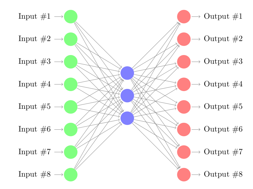
Below is the schematic structure of an auto-encoder with a single hidden layer. The vectors \(\mathcal{X}\) are of length \(d=8\) and we attempt to reduce the dimensionality of the inputs to \(p=3\).
Using Auto Encoders for Anomaly Detection
The idea to apply it to anomaly detection is very straightforward:
- Train an auto-encoder on \(\mathcal{X}_{train}\) with good regularization (preferrably recurrent if \(\mathcal{X}\) is a time process).
- Evaluate it on the validation set \(\mathcal{X}_{val}\) and visualise the reconstructed error plot (sorted).
- Choose a threshold -like 2 standard deviations from the mean- which determines whether a value is an outlier (anomalies) or not. This threshold can by dynamic and depends on the previous errors (moving average, time component).
Examples
Example 1: distance-based outliers generation and detection
Lets assume the same matrix \(\mathcal{X} \in \mathbb{R}^{dt} \sim \mathcal{MVN}(0,\Sigma_t)\) where \(\Sigma_t = I\), \(X^i_t\) is independent of \(X^j_t\) for \(i \neq j\) and for a given \(t\). Also, we replace \(N\) percent of the generated values of \(\mathcal{X}\) by outliers, whose values lay in an unlikely range of the standard normal distribution (say 6 to 9). The set of outliers is denoted by \(\mathcal{O}\).
Note that \(\mathcal{O}\) was selected in such a way that it is highly improbable to sample such values with a standard normal sampling: \(P(X^k > 6) << 1\). We bound this interval to 9 to keep the same order of magnitude in our dataset.
The goal is to find the time indices \(t_{o1}, ..., t_{on}\) of the outliers in the augmented matrix \(\mathcal{X}\).
We find an accuracy of 1, hit rate of 1 and precision of 1. The system is very well-suited for this particular task. The code is available here: https://gist.github.com/philipperemy/b8a7b7be344e447e7ee6625fe2fdd765.
Example 2: Multivariate normal distribution with nonidentity covariance matrix
In this section, we consider two cases:
- Case 1: Intra covariance (related to the dimension \(d\)). It is assumed here that all the samples are i.i.d. There is no time dependency. \(\Sigma_t \neq I\) for any \(t > 0\).
- Case 2: Time covariance (related to the dimension \(t\)). Here, the process is assumed to have a non-zero auto-correlation function. \(\Sigma_t = I\) for all \(t > 0\).
The idea is to be able to capture covariance changes inside the data and over time. We recall the definition of the covariance below for conveniency.
Covariance is a measure of how much two random variables change together. If the greater values of one variable mainly correspond with the greater values of the other variable, and the same holds for the lesser values, i.e., the variables tend to show similar behavior, the covariance is positive. The covariance matrix generalizes the notion of covariance to multiple dimensions.
Case 1: Covariance along the dimension \(d\)
Let’s generate 10000 samples of the \(d=\)100-dimensional MVN process \(X\) with a covariance matrix \(\Sigma = \Sigma_{train}\). This will be our training set.
Let’s now generate twice the number of samples (20000) for our testing set. The first half has a covariance matrix denoted \(\Sigma_{test} \neq \Sigma_{train}\) and the second half has the same covariance as the training set: \(\Sigma_{train}\).
We expected the loss inequality: \(L_{test, \Sigma_{test}} > L_{test, \Sigma_{train}}\) because the second half of the testing set is generated from the training set generator.
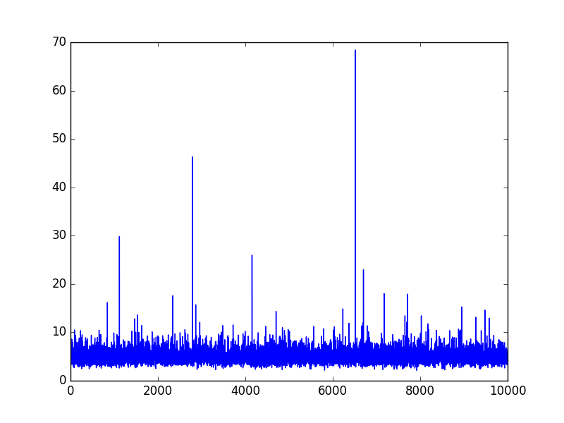
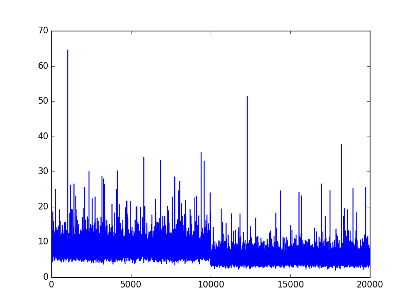
With little surprise, we find that the MSE is lower in the second half of the testing and corresponds thoroughly to the MSE of the training set. The model is capable of distinguishing when the covariance matrix changes.
Case 2: Covariance across the dimension \(t\) (only)
We consider an auto regressive process of order AR(1) to model this non-zero autocorrelation function:
\[X_{t}=c+\varphi X_{t-1}+\epsilon_{t}\]where \(\epsilon_t\) is a white noise process with zero mean and constant variance \({\displaystyle \sigma _{\varepsilon }^{2}}\).
The autocovariance is given by (where \(n\) is the lag):
\[B_n=E(X_{t+n}X_{t})-\mu^2= \frac{\sigma_{\epsilon}^2}{1-\varphi^2} \varphi ^{|n|} = f(\varphi^2, \sigma_{\epsilon}^2, |n|)\]Throughout this setup, we fix \(d=1\) for sake of simplicity. The problem remains exactly the same and becomes simpler to visualise and understand.
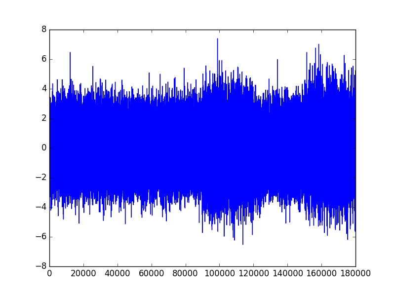
The noise is generated from a standard normal distribution. \(X\) is split into two main segments: \(X_{train}\) and \(X_{test}\).
On the training part \(X_{train}\), we have \(\varphi = \phi_1\), constant. We split the testing set \(X_{test}\) into 3 equally-length segments where we have \(\varphi = \phi_2 (\neq \phi_1)\) for the first segment, \(\phi_1\) for the second one, and \(\phi_2\) for the third one.
We can summarize the process generation this way:
\[X = (X_{train}, X_{test}) = (X(\phi_1), X(\phi_2) \cup X(\phi_1) \cup X(\phi_2))\]The goal here is to detect the regime shifts of the process \(X\) for different values of \((\phi_1, \phi_2)\).
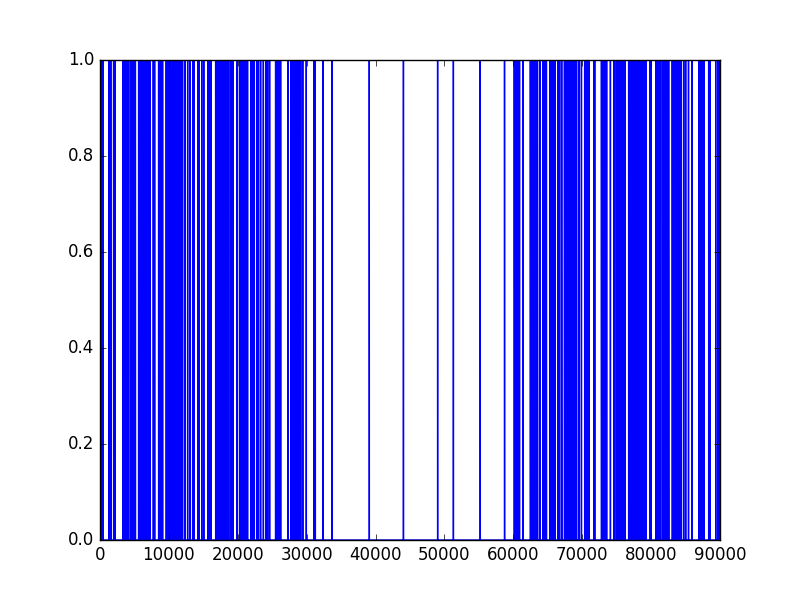
In this example, we set \(|X| = 180000, |X_{train}| = 90000, |X_{test}| = 90000.\) \(X_{train}\) comes before \(X_{test}\).
Results for \((\phi_1, \phi_2) = (0.4, 0.8)\)
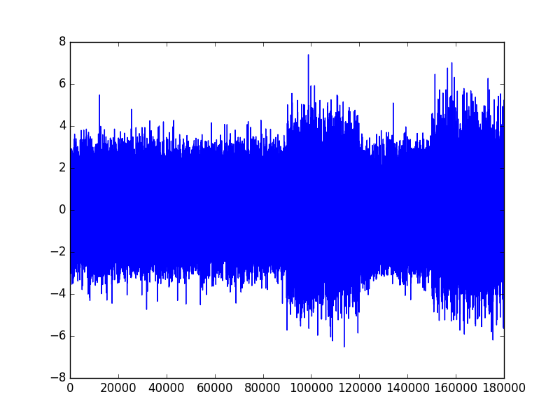
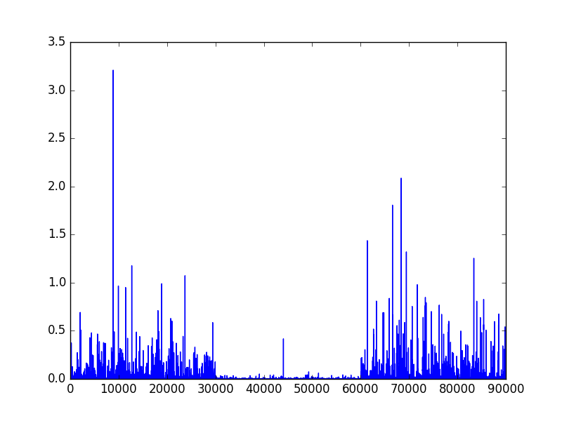
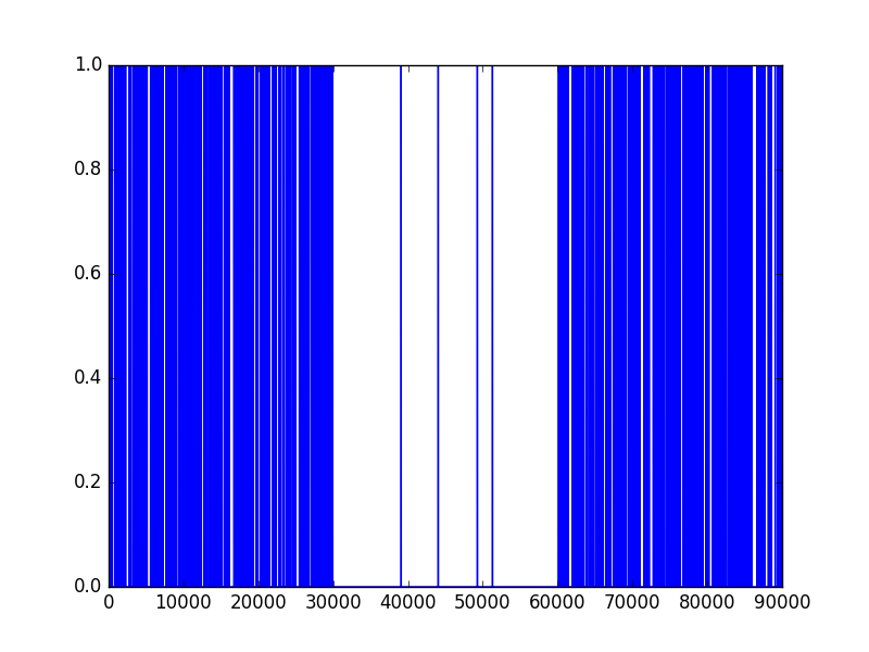
Not surprisingly, the model appears to be almost flawless and can detect accurately a change in the parameter \(\varphi\). Let’s see if it still performs well if we decrease the quantity \((\phi_{2} - \phi_{1})^2\).
Results for \((\phi_1, \phi_2) = (0.6, 0.8)\)
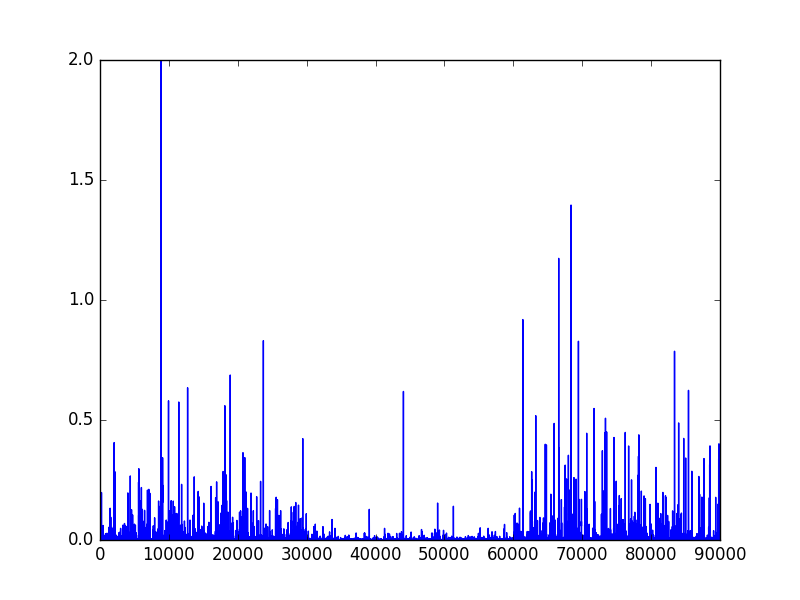
When the difference between \(\phi_1\) and \(\phi_2\) is only 0.2, the model can still figure out the regime shift accurately.
IMPORTANT NOTE: The choice of the loss function is very important and in most of the cases, the MSE might not be the most adapted measure. For example, let’s assume that we train on any zero-centered signal with the outliers be zero-valued. The MSE of the outliers is very likely to be less than the MSE of our original signal (because the signal is centered around 0, the value of the outliers - 0 here - equal the expected value of the signal). In this case, the MSE is unable to classify between our signal and the outliers. In this case, we can add a moving average component to the MSE and we look at the deviations from the moving average for outlier detection. Also, looking at the first order derivatives of the MSE (rate of change) could be beneficial to the analysis.
Conclusion
Throughout this article, we presented straightforward toy examples to be more familiar to auto encoders (MLP, LSTM…). Keep in mind that real world problems are usually very different from the content of the examples mentioned above.
However, we are utterly convinced that the auto encoders remain a powerful dimensionality reduction tool for non linear problems.