
Bayesian Optimization Example
In this article, I will present a very useful technique to find the global maximum of any function \(f : \mathbb{R}^n \rightarrow \mathbb{R}\). It is called Bayesian Optimization.
I will use this very good Bayesian Optimization framework.
Let us begin by a brief recap of what is Bayesian Optimization and why many people use it to optimize their models.
Bayesian Optimization is a constrained global optimization package built upon bayesian inference and gaussian process, that attempts to find the maximum value of an unknown function in as few iterations as possible. This technique is particularly suited for optimization of high cost functions, situations where the balance between exploration and exploitation is important.
Instead of attacking BO from a theoretical point of view, I think it is definitely easier to understand it with a short example. I have selected an analytic function (defined below) and lets see if we can find its global maximum.
First of all, let us start by installing the required packages (for those who dont want to mess up their python setup, please consider using the Virtual Environments in Python.
pip install numpy scipy scikit-learn bayesian-optimization
From there, lets proceed step by step.
from bayes_opt import BayesianOptimization
import numpy as np

import matplotlib.pyplot as plt
from matplotlib import gridspec
%matplotlib inline
Target Function
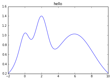
The function we will analyze today is a 1-D function with multiple local maxima: \(f(x) = e^{-(x - 2)^2} + e^{-\frac{(x - 6)^2}{10}} + \frac{1}{x^2 + 1},\). Its maximum is at \(x = 2\) and we assume that we already know that the maximum is in \(x \in (-2, 10)\).
def target(x):
    return np.exp(-(x - 2)**2) + np.exp(-(x - 6)**2/10) + 1/ (x**2 + 1)
KAPPA = 5
x = np.linspace(-2, 10, 1000)
y = target(x)

plt.plot(x, y)
Create a BayesianOptimization Object
A minimum number of 2 initial guesses is necessary to kick start the algorithms, these can either be random or user defined.
bo = BayesianOptimization(target, {'x': (-2, 10)})
In this example we will use the Upper Confidence Bound (UCB) as our utility function. It has the free parameter \(\kappa\) which control the balance between exploration and exploitation; we will set \(\kappa=5\) which, in this case, makes the algorithm quite bold. Additionally we will use the cubic correlation in our Gaussian Process.
gp_params = {'corr': 'cubic'}
bo.maximize(init_points=2, n_iter=0, acq='ucb', kappa=KAPPA, **gp_params)
Plotting and visualizing the algorithm at each step
Two random points
After we probe two points at random, we can fit a Gaussian Process and start the bayesian optimization procedure. Two points should give us a uneventful posterior with the uncertainty growing as we go further from the observations.
After one step of GP (and two random points)
bo.maximize(init_points=0, n_iter=1, kappa=KAPPA)
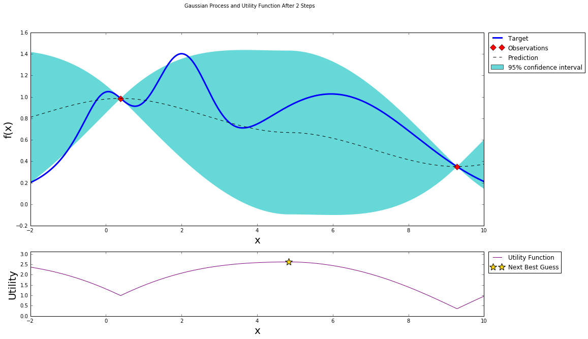
After two steps of GP (and two random points)
bo.maximize(init_points=0, n_iter=1, kappa=KAPPA)
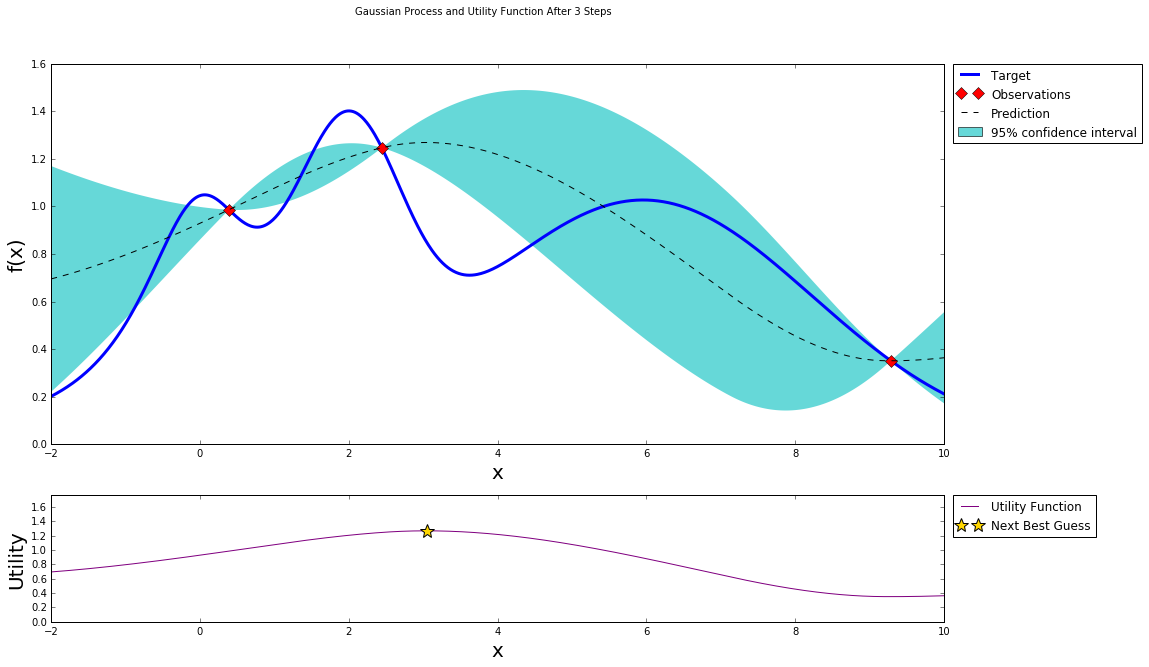
After three steps of GP (and two random points)
bo.maximize(init_points=0, n_iter=1, kappa=KAPPA)
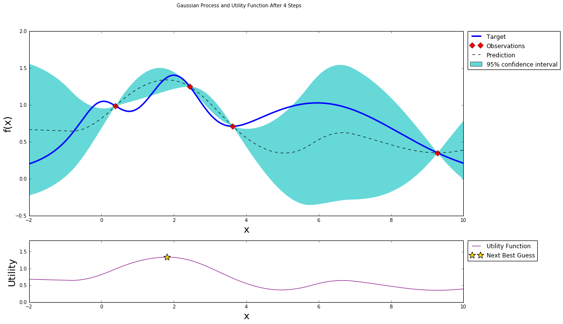
After four steps of GP (and two random points)
bo.maximize(init_points=0, n_iter=1, kappa=KAPPA)
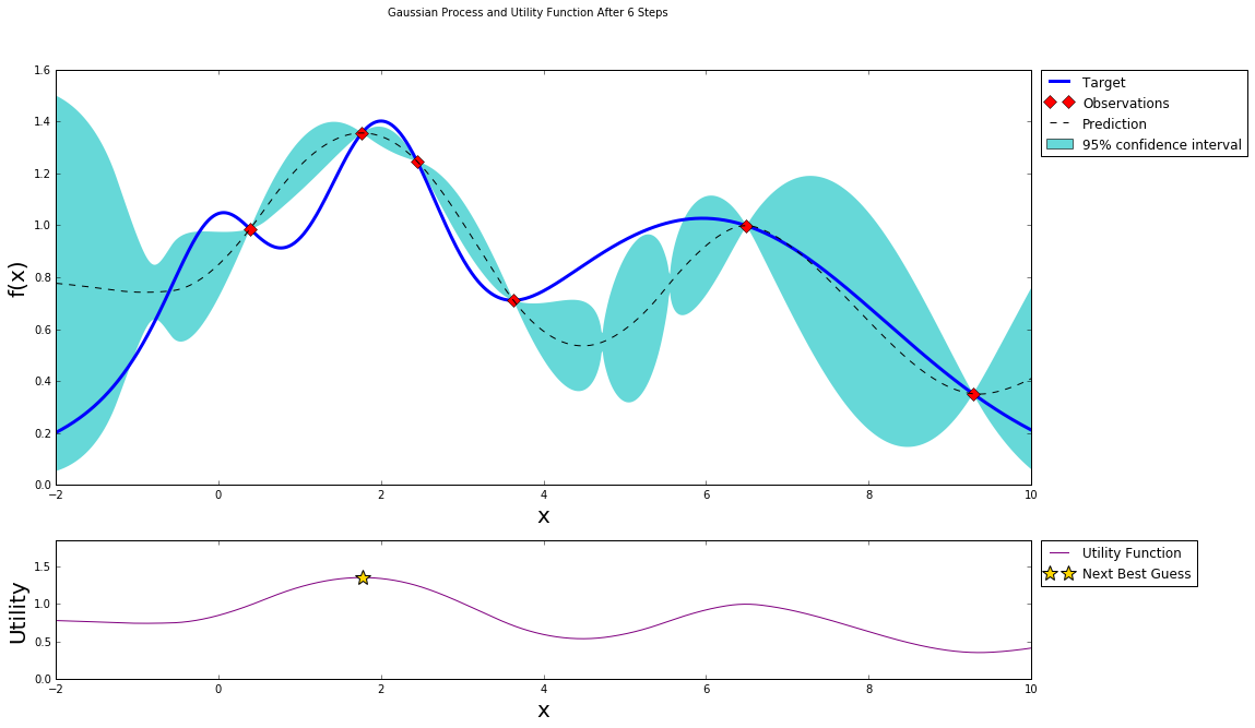
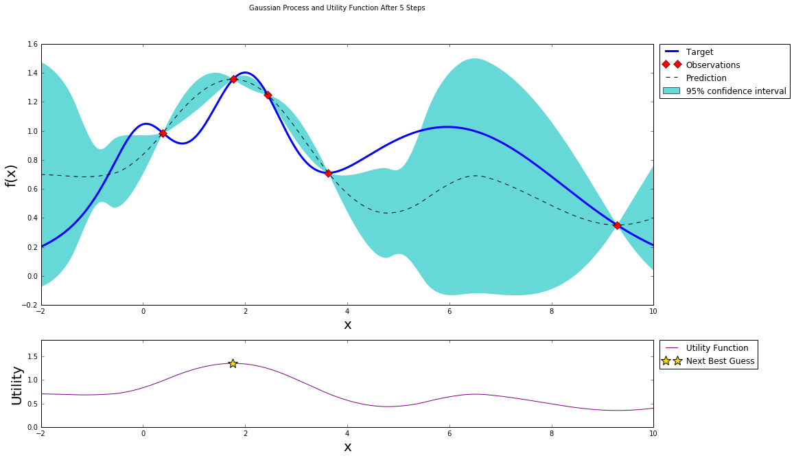
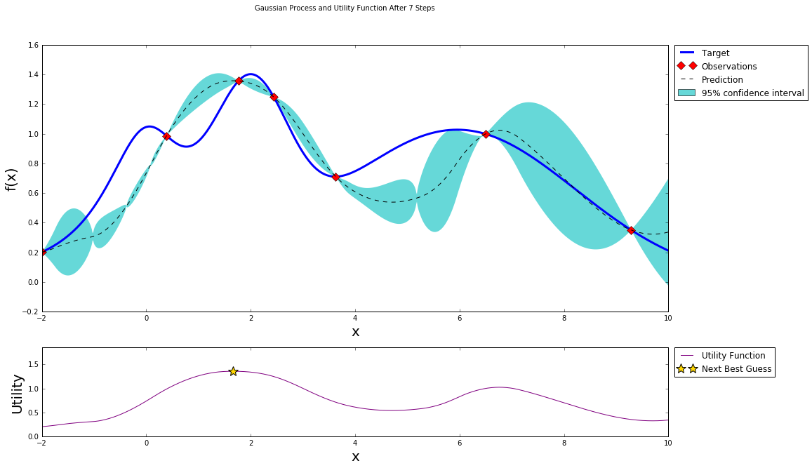
After five steps of GP (and two random points)
bo.maximize(init_points=0, n_iter=1, kappa=KAPPA)
Stopping
After just a few points the algorithm was able to get pretty close to the true maximum. It is important to notice that the trade off between exploration (exploring the parameter space) and exploitation (probing points near the current known maximum) is fundamental to a succesful bayesian optimization procedure. The utility function being used here (Upper Confidence Bound - UCB) has a free parameter \(\kappa\) that allows the user to make the algorithm more or less conservative. Additionally, a the larger the initial set of random points explored, the less likely the algorithm is to get stuck in local minima due to being too conservative.
All the source code is available on the repository at https://github.com/fmfn/BayesianOptimization.