The idea of this post is to provide a brief and clear understanding of the stateful mode, introduced for LSTM models in Keras. If you have ever typed the words lstm and stateful in Keras, you may have seen that a significant proportion of all the issues are related to a misunderstanding of people trying to use this stateful mode. This post attempts to give insight to users on how to use for their applications.

I am not going to go into details on how Recurrent Neural Networks work. For this, I strongly suggest you to check the fantastic article made by Colah Understanding LSTM Networks.

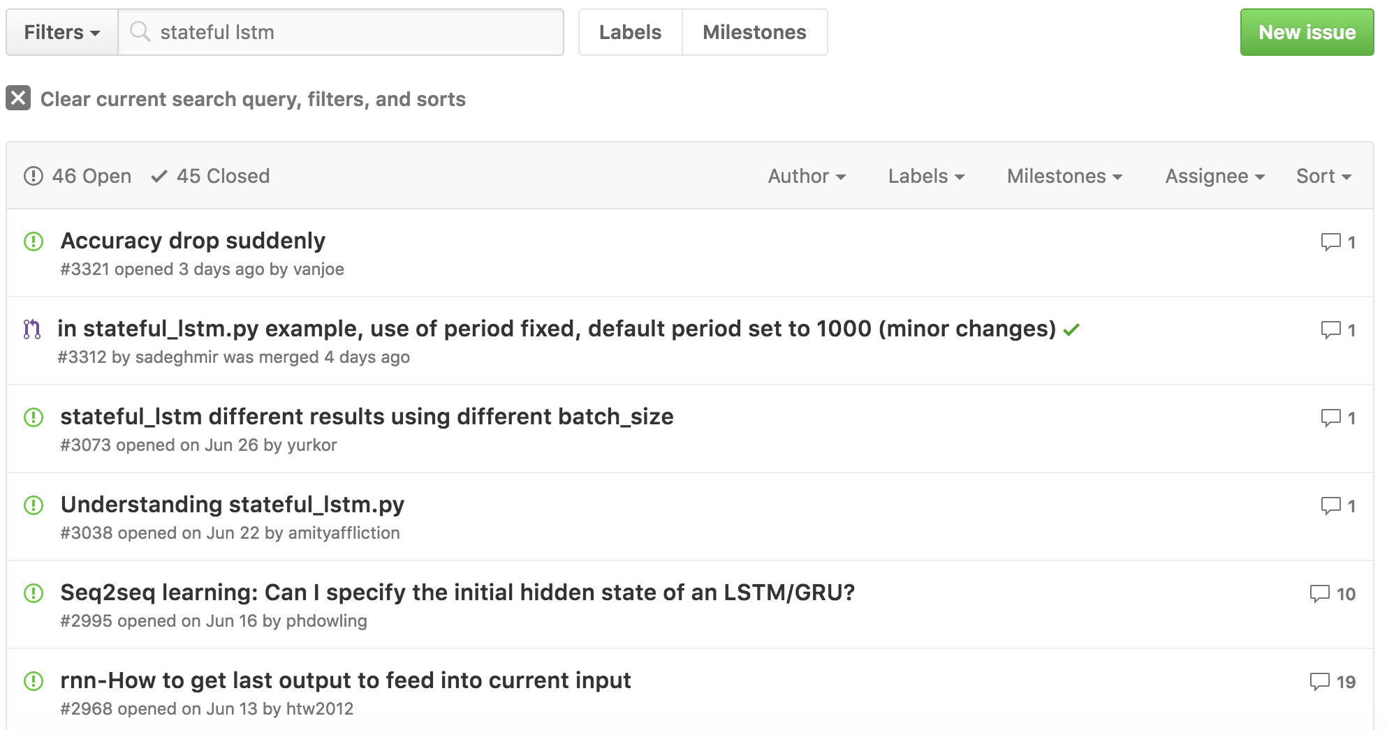Screenshot of the issues related to stateful LSTM in Keras

Introduction of Stateful LSTMs

In Recurrent Neural Networks, we are quickly confronted to the so-called gradient vanishing problem:

In machine learning, the vanishing gradient problem is a difficulty found in training artificial neural networks with gradient-based learning methods and backpropagation. In such methods, each of the neural network’s weights receives an update proportional to the gradient of the error function with respect to the current weight in each iteration of training. Traditional activation functions such as the hyperbolic tangent function have gradients in the range \((−1, 1)\) or \([0, 1)\), and backpropagation computes gradients by the chain rule. This has the effect of multiplying n of these small numbers to compute gradients of the “front” layers in an n-layer network, meaning that the gradient (error signal) decreases exponentially with n and the front layers train very slowly.

One solution is to consider adding the updates instead of multiplying them, and this is exactly what the LSTM does. The state of every cell is updated in an additive way (Equation 9) such that the gradient hardly vanishes.

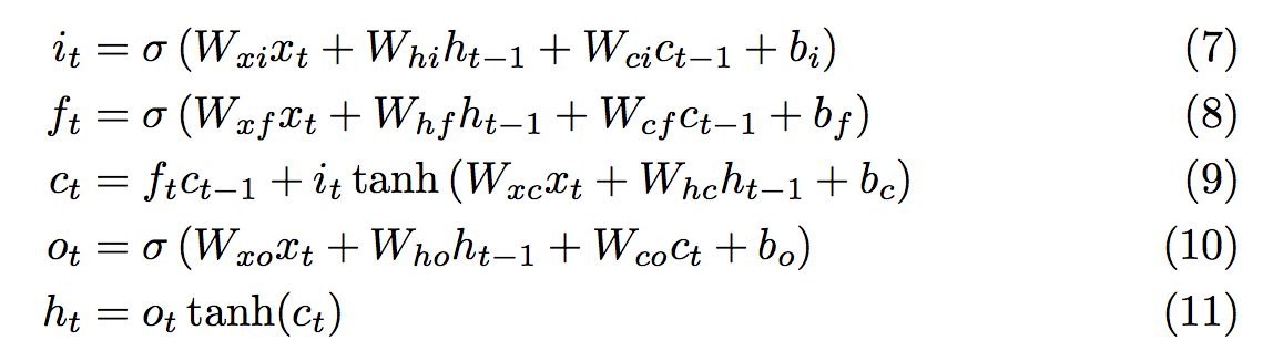Equations of the LSTM model in Graves paper

The documentation of Keras for Recurrent Layers is well written and available here : http://keras.io/layers/recurrent/. However I think it lacks of some self-explanatory examples and some corner cases to develop a strong understanding. Let’s first start by setting up some general questions:

Questions and Answers

• I’m given a big sequence (e.g. Time Series) and I split it into smaller sequences to construct my input matrix \(X\). Is it possible that the LSTM may find dependencies between the sequences?
  No it’s not possible unless you go for the stateful LSTM. Most of the problems can be solved with stateless LSTM so if you go for the stateful mode, make sure you really need it. In stateless mode, long term memory does not mean that the LSTM will remember the content of the previous batches.

• Why do we make the difference between stateless and stateful LSTM in Keras?
  A LSTM has cells and is therefore stateful by definition (not the same stateful meaning as used in Keras). Fabien Chollet gives this definition of statefulness:
  stateful: Boolean (default False). If True, the last state for each sample at index i in a batch will be used as initial state for the sample of index i in the following batch.
  
  Said differently, whenever you train or test your LSTM, you first have to build your input matrix \(X\) of shape nb_samples, timesteps, input_dim where your batch size divides nb_samples. For instance, if nb_samples=1024 and batch_size=64, it means that your model will receive blocks of 64 samples, compute each output (whatever the number of timesteps is for every sample), average the gradients and propagate it to update the parameters vector.
  
  By default, Keras shuffles (permutes) the samples in \(X\) and the dependencies between \(X_i\) and \(X_{i+1}\) are lost. Let’s assume there’s no shuffling in our explanation.
  
  If the model is stateless, the cell states are reset at each sequence. With the stateful model, all the states are propagated to the next batch. It means that the state of the sample located at index \(i\), \(X_i\) will be used in the computation of the sample \(X_{i+bs}\) in the next batch, where \(bs\) is the batch size (no shuffling).

• Why do Keras require the batch size in stateful mode?
  When the model is stateless, Keras allocates an array for the states of size output_dim (understand number of cells in your LSTM). At each sequence processing, this state array is reset.
  
  In Stateful model, Keras must propagate the previous states for each sample across the batches. Referring to the explanation above, a sample at index \(i\) in batch #1 (\(X_{i+bs}\)) will know the states of the sample \(i\) in batch #0 (\(X_i\)). In this case, the structure to store the states is of the shape (batch_size, output_dim). This is the reason why you have to specify the batch size at the creation of the LSTM. If you don’t do so, Keras may raise an error to remind you: If a RNN is stateful, a complete input_shape must be provided (including batch size).

Self-explanatory Examples of Stateful LSTMs

Let’s consider the easiest example where batch_size=1 and shuffle=False to avoid any confusions.

Let the input matrix \(X\) be of the arbitrary shape \((1200, 20)\). Those values are totally arbitrary, trust me! Let’s also assume that \(X\) is made exclusively of zeros except in the first column where exactly half of the values are 1.

N_train = 1000
from numpy.random import choice
one_indexes = choice(a=N_train, size=N_train / 2, replace=False)
X_train[one_indexes, 0] = 1  # very long term memory.

The first column is also stored in \(Y\) and it will be the target of the model. In other words, our model must understand that if the first value of the sequence is 1, then the result is 1, 0 otherwise.

We split \((X, Y)\) in training (1000 rows) and validation sets (200 rows).

Now that we have the setup, let’s try to illustrate each point that we have discussed above.

Impact of sequences subsampling

We consider a stateless LSTM in our first experiment and our dataset \((X, Y)\). Our objective is to prove that if we split the big sequences contained in \(X\) into smaller sequence, the model cannot converge. The function that we use to split a big sequence into subsequences is:

def prepare_sequences(x_train, y_train, window_length):
    windows = []
    windows_y = []
    for i, sequence in enumerate(x_train):
        len_seq = len(sequence)
        for window_start in range(0, len_seq - window_length + 1):
            window_end = window_start + window_length
            window = sequence[window_start:window_end]
            windows.append(window)
            windows_y.append(y_train[i])
    return np.array(windows), np.array(windows_y)

As an example, if we have \(X = [1, 0, 0, 0, 0]\), \(Y = 1\) and if window_length=2, the output will be:

\(X_{out} = [[1, 0], [0, 0], [0, 0], [0, 0]]\), \(Y_{out} = [1, 1, 1, 1]\). The operation is not destructive but reversible. We repeat the procedure for every \((X_i, Y_i)\) to re create our new matrices \((X, Y)\) that will used as inputs to the LSTM.

With window_length=10, the shapes become:

x_train shape: (11000, 10, 1)
y_train shape: (11000, 1)
x_test shape: (2200, 10, 1)
y_test shape: (2200, 1)

instead of (without subsequences sampling):

x_train shape: (1000, 20, 1)
y_train shape: (1000, 1)
x_test shape: (200, 20, 1)
y_test shape: (200, 1)

Indeed in a sequence of length \(20\), we have exactly \((20-10+1)\) sequences of length \(10\) (sketch it if you’re not convinced). Because we have \(1000\) samples (sequences) in the training set, we have \(1000*11 = 11000\) subsequences in our resulting training set (we make sure to keep the order). Let’s feed that to our LSTM:

print('Building STATELESS model...')
model = Sequential()
model.add(LSTM(10, input_shape=(max_len, 1), return_sequences=False, stateful=False))
model.add(Dense(1, activation='sigmoid'))
model.compile(loss='binary_crossentropy', optimizer='adam', metrics=['accuracy'])
model.fit(X_train, y_train, batch_size=batch_size, nb_epoch=15,
          validation_data=(X_test, y_test), shuffle=False)
score, acc = model.evaluate(X_test, y_test, batch_size=batch_size, verbose=0)

Because the targets \(Y\) are approximately equally distributed (half are 0, half are 1), the baseline is an accuracy of 0.5.

After 15 epochs, on this very simple task, we have:

Epoch 15/15 11000/11000 [==============================] - 21s - loss: 0.6623 - acc: 0.5343 - val_loss: 0.6606 - val_acc: 0.5455

The interpretation of this result is very clear. The LSTM cannot find the optimal solution when working with subsequences. On such an easy problem, we expect an accuracy of more than 0.99.

Activating the statefulness of the model does not help at all (we’re going to see why in the next section):

model.add(LSTM(10, batch_input_shape=(batch_size, max_len, 1), return_sequences=False, stateful=True))

Epoch 15/15 11000/11000 [==============================] - 20s - loss: 0.6964 - acc: 0.5222 - val_loss: 0.7046 - val_acc: 0.5000

As a conclusion, subsampling does not help the LSTM converge. So when you have a big time series (e.g. in financial markets), the lookback window length is crucial and can be found with Bayesian Optimization .

Mastering stateful models

Let’s consider the setup without sequences subsampling where the dimensions of our input matrices are:

x_train shape: (1000, 20, 1)
y_train shape: (1000, 1)
x_test shape: (200, 20, 1)
y_test shape: (200, 1)

Also to make things easier, we consider batch_size=1. Our stateful model looks like this:

print('Build STATEFUL model...')
model = Sequential()
model.add(LSTM(10, batch_input_shape=(1, 1, 1), return_sequences=False, stateful=True))
model.add(Dense(1, activation='sigmoid'))
model.compile(loss='binary_crossentropy', optimizer='adam', metrics=['accuracy'])

The idea is to split each sequence \(X_i\) (of length \(20\)) into elements of size \(1\) and feed them to the LSTM. Once the sequence is over, we manually reset the states of the LSTM to have a clean setup for the next one. For each element, we associate the related target \(Y_i\).

For instance, if we have \(X_i = [1, 0, 0 ..., 0]\) and \(Y_i = [1]\), we feed \(((x_{i0}=[1], y_i=[1])\), \((x_{i1}=[0], y_i=[1])\),…, \((x_{i20}=[0], y_i=[1]))\) to the LSTM.

The operation is not destructive but reversible. We repeat the procedure for every \((X_i, Y_i)\) to re create our new matrices \((X, Y)\) that will used as inputs to the LSTM.

Because the LSTM is stateful, the state will be propagated to the next batch. Also because the batch_size=1, we are sure that the state of the last element will be used as input to the current element. The code is available below and is a bit more involved:

print('Train...')
for epoch in range(15):
    mean_tr_acc = []
    mean_tr_loss = []
    for i in range(len(X_train)):
        y_true = y_train[i]
        for j in range(max_len):
            tr_loss, tr_acc = model.train_on_batch(np.expand_dims(np.expand_dims(X_train[i][j], axis=1), axis=1),
                                                   np.array([y_true]))
            mean_tr_acc.append(tr_acc)
            mean_tr_loss.append(tr_loss)
        model.reset_states()

    print('accuracy training = {}'.format(np.mean(mean_tr_acc)))
    print('loss training = {}'.format(np.mean(mean_tr_loss)))
    print('___________________________________')

    mean_te_acc = []
    mean_te_loss = []
    for i in range(len(X_test)):
        for j in range(max_len):
            te_loss, te_acc = model.test_on_batch(np.expand_dims(np.expand_dims(X_test[i][j], axis=1), axis=1),
                                                  y_test[i])
            mean_te_acc.append(te_acc)
            mean_te_loss.append(te_loss)
        model.reset_states()

        for j in range(max_len):
            y_pred = model.predict_on_batch(np.expand_dims(np.expand_dims(X_test[i][j], axis=1), axis=1))
        model.reset_states()

    print('accuracy testing = {}'.format(np.mean(mean_te_acc)))
    print('loss testing = {}'.format(np.mean(mean_te_loss)))
    print('___________________________________')

Let’s see how the accuracy behaves in the same with our stateful model. As expected, after just a few epochs, our accuracy is very close to 1, which means that our model could successfully catch the pattern.

epoch = 1, accuracy training = 0.997300028801, accuracy testing = 1.0
epoch = 2, accuracy training = 1.0, accuracy testing = 1.0

Finally, let’s see how the stateless model would perform here:

model.add(LSTM(10, batch_input_shape=(1, 1, 1), return_sequences=False, stateful=False))

epoch = 1, accuracy training = 0.53409999609, accuracy testing = 0.524999976158
epoch = 2, accuracy training = 0.535149991512, accuracy testing = 0.524999976158

Not surprisingly, the model cannot converge because the state is not propagated across the elements.

The code was a bit more difficult to write because we have to manually call model.reset_states() at each new sequence processed. Another method to do that is to write a callback that reset the states at each sequence like this:

max_len = 20
class ResetStatesCallback(Callback):
    def __init__(self):
        self.counter = 0

    def on_batch_begin(self, batch, logs={}):
        if self.counter % max_len == 0:
            self.model.reset_states()
        self.counter += 1
        
x = np.expand_dims(np.expand_dims(X_train.flatten(), axis=1), axis=1)
y = np.expand_dims(np.array([[v] * max_len for v in y_train.flatten()]).flatten(), axis=1)
model.fit(x, y, callbacks=[ResetStatesCallback()], batch_size=1, shuffle=False)

Build STATEFUL model...
Epoch 1/10
20000/20000 [==============================] - 29s - loss: 0.0256 - acc: 0.9921    
Epoch 2/10
20000/20000 [==============================] - 29s - loss: 2.2883e-07 - acc: 1.0000 

Note: be careful as it seems that the callbacks are not properly called when using the parameter validation_data in model.fit(). You may have to do your validation/testing manually by calling predict_on_batch() or test_on_batch().

Throughout this article, we came up with several toy examples that illustrate how to use stateful LSTM. Don’t forget to comment if you see any mistakes or some ways of improving the code.